1. Introduction

Radar stands for Radio Detection and Ranging. It refers to the use of radio waves to detect objects and determine the distance (range) to the object.

Radio transmissions were employed for the first time by Marconi in 1896, and subsequently used for various types of information transfer. In 1897 Marconi sent a signal from the Isle of Wight, near England, to North America. Experimental scientists also used the new tool to study the newly discovered "ionosphere", which was capable of reflecting these radio waves.

Radar itself uses radio waves, but requires some extra complexity. Originally developed for detection of enemy aircraft and vehicles during World-War II, it subsequently evolved into much more, and has been used in many scientific experiments in the past 60 years. No longer is it restricted to detection of "hard" targets like aircraft, but can be used to detect targets like raindrops, and even turbulence in the atmosphere. Similar principles have even been developed using laser-light instead of radio waves (lidar), and also for acoustic waves (sodar), but we will concentrate here on radar.

Some of the most common platforms used for meteorological studies include ground stations, rockets, ships, blimps, tall towers and balloons, but radars are a key tool. Some typical platforms are shown in the attached diagram. (click the diagram to see an enlarged version).

Radars, however, will be our focus here. They have particularly become important in meteorology because of the following reasons.

(i) They can see through fog, cloud, rain and other types of atmospheric conditions which light cannot pass through.

(ii) They can observe many places in the sky almost simultaneously.

(iii) They can run continuously, often without operators being present (computer controlled).

(iv) They can operate during both day and night.

(v) The data from them can be easily stored to computer and then subjected to many types of sophisticated analysis.

(vi) Modern solid-state radars often need little maintenance, or replacement of parts, so the largest expense is often the setup costs.

(vii) Radars are not restricted to ground-level studies, and can often observe several kilometres upward into the atmosphere.

We will shortly discuss the principles of radar theory in descriptive terms. However, before doing so, it is worth noting that there are many different types of radar, using different designs. Some examples of different antennas are shown below. (click the diagrams to see enlarged versions).

Typical side-looking dish radar.
The first diagram shows the dish-antenna, which rotates around in a full circle several times per minute. Such dishes are usually housed in fibre-glass domes, as shown in the second and third figures, in order to protect the dishes from the rain and wind. This is possible because radio waves can pass right through fibre-glass.

Larger side-looking dish radar.
This picture shows a larger side-looking weather radar which is too big to be enclosed in a fibre-glass dome. This radar is a so-called S-band radar, operated by NCAR (National Center for Atmospheric Research) in the USA.

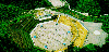
Sondrestrom Radar.
This radar is primarily used for studying the ionosphere and middle atmosphere, and is situated in Greenland. It is especially used to study the aurora, and a green aurora appears in the background of the picture. You can see other instruments situated near the radar, including the green beam from a lidar shooting upward from the main building.

Arecibo Radio Dish.
This radio telescope is best known for it applications in astronomy, including investigations of the planets and galaxies. However, it has also been used for atmospheric studies of the ionosphere, mesosphere, stratosphere and troposphere.

"FMCW" mobile radar.
In addition to large radars, smaller, portable ones can also be useful. This picture shows a powerful portable radar designed specifically to study the lowest few hundred metres of the atmosphere (the boundary layer) at extremely high resolution (from Eaton et al., Radio Sci., vol 30, p 75, 1995). This radar works at much higher frequencies than the ones shown above.

Another portable radar.
Portable radars are also very useful for studying mobile weather conditions like tornadoes. This particular radar is being operated by graduate students from the University of Oklahoma ( Bull. American Meteorol. Soc., vol 70, 1989).

Japanese "MU" {"Middle and Upper atmosphere) radar. Antennas within the MU radar.
This is an example of a "windprofiler" radar - this one is currently the most expensive one of its type in the world. It is situated in Japan. The first diagram shows an aerial view, while the second shows a view of the antennas within the main array. The principles of windprofiler radars will be discussed shortly. I am going to show several different pictures of windprofiler radars, because these radars have the most diverse designs of any radars. This is because these instruments are still under development, so each new group of researchers who builds one tends to experiment with different designs.

Here are some other windprofiler radars

The windprofiler and ionospheric radar near Jicamarca, Peru. This is an extremely famous radar in the field of windprofiler research, for it was with this radar that scientists (specifically Dr. Ronald Woodman and one of his colleagues, A. Guillen), first discovered that radars working at frequencies of around 50 MHz could be used for tropospheric and stratospheric studies of the atmosphere. Previously, the radar had been used only for ionospheric work. This discovery laid the foundation for the field of windprofiler studies.

The Andennes windprofiler radar in Norway This photograph shows yet another type of windprofiler design - this time for a radar at Andenes in northern Norway. It is operated by the Institute for Atmospheric Physics in Germany.

The CLOVAR radar in Canada. The CLOVAR radar at sunset. These pictures show views of the radar built and operated by this particular author. It is owned by the University of Western Ontario in Canada.

Resolute Bay windprofiler radar. This pictures show a view of another radar built and operated by this particular author. This one exists at Resolute Bay in Nunavut, Canada.

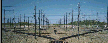
Poker Flat radar. This shows another radar using a different antenna design. In this case the antennas are comprised of so-called "coaxial-coaxial" (co-co) antennas. They consists of lines of coaxial cables joined up in a special way. The cables are coupled together in increments of length equal to one half of a wavelength. These cables can be (just) seen running horizontally across the picture atop of the stakes in the ground, at about the same level as the man standing in the picture. This radar was situated at Poker Flat in Alaska, but has since been dis-assembled.

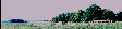
Piura radar, Peru. This shows another radar using a co-co design. In this case the radar is situated at Piura in Peru.

Wind profiler, Lindenberg, Germany. Another windprofiler radar design. This radar works at a higher frequency than those above namely at around 480 MHz. Many of the windprofilers shown above work at around 50 MHz.

Boundary Layer radar, McGill University. A further outgrowth of windprofiler studies was the demonstration that atmospheric radar scatter could be utilized at frequencies as high as 1000 MHz in the so-called "windprofiler mode". This radar is a system that works at 900 MHz, and is designed to probe the lowest few hundred metres of the atmosphere, and up to a couple of kilometres in height. These radars are small and portable.

Boundary Layer radar, Lindenberg. Another example of a boundary layer radar. Some of these radars also have a special feature added to them called RASS, which stands for Radio Acoustic Sounding System. By utilizing this system, the radar can be used to measure the speed of sound in air as a function of height, and therefore the temperature as a function of height can be determined.

There are many different radars, but hopefully this has given you a flavour of the variety available.

I now want to go on to discuss the fundamental principles of radar. These principles are common to all of the above systems.

2. The Principles of Radar.

In the following sections, I will discuss the basic principles of radar application. I will keep the discussion descriptive, and avoid mathematics, where-ever I can. We will start by looking at the distribution of power radiated from a radar dish or array.

2(i) Power Distribution

If you are used to looking at light beams, you probably expect a "beam" of light to be a narrow line looking something like that shown in this picture, where you can see a green laser beam pointing up into the sky. But with the transmission from a radar dish, things look quite different. The radiation is emitted over a range of angles, with strongest power near the centre of the beam, and diminishing power as one moves out. An illustration of this effect is shown in this diagram, where the amount of radiation emitted is greater where the shading is darkest. There is no sharp edge to the beam. (The diagram shows some points where the shading seems to change abruptly, but that is just my poor artwork! The shading should grade smoothly from the darkest to the lightest greys as one moves out from the centre.) The width of the central portion is different for different radars, being more than 10 degrees in some cases, and less than 1 degree in others. The pattern which describes the radiated power as a function of angle is called the "polar diagram", and the width of the central region is defined as the beam-width. To be precise, the beam width is normally defined as the angle from the point where the radiated power falls to one half of the maximum on one side of the beam, to the identical point on the other side of the beam. (Some authors use the angle between one-quarter power points). The region of radiation which falls between these limits is referred to as the "beam" of the radar, but it is important to remember that it does not have a sharp cut-off at its edges.

The beam-width in fact is proportional to the value of the radar wavelength divided by the diameter of the radar dish (or width of the array in the case of a phased-array radiating and receiving system).

There is one other feature about the radar beam pattern which I have not represented in the above diagram, and this is the existence of "side-lobes". While I have drawn the power density to decrease smoothly with increasing angular distance from the centre of the beam, it in fact turns out that every now and then the power rises for a short range of angles, then falls away, then rises again, then falls, etc. These "local increases" in power are called sidelobes. They never rise as high in power density as the main part of the beam, but it is important to know about them in any serious examination of a radar system.

You might now ask - why do radars "smear out" the signal like this, and have sidelobes, but laser beams do not? Well, in fact laser beams do show these same effects - collectively they are called diffraction. However, diffraction is not as evident with the laser beams, because the wavelength of light is many times less than for radio waves. It turns out that typically the ratio of the diameter of the mirror of a lidar to the wavelength of the light is many times greater than the ratio of the diameter of the radar dish to the radar wavelength, so the "spread" of the light beam is almost imperceptible.

2(ii) The Principle of Range Determination

We have now demonstrated the lateral spread of the radar signal. The next thing is to look at the situation as the radiation propagates along the beam.

The majority of (but not all) atmospheric radars use so-called pulsed radars. This involves the radars transmitting pulses of radio waves at regular intervals - typically with times between transmissions of the order of milliseconds and less. The "pulse Repetition Frequency" (PRF) refers to the number of pulses transmitted per second, and can vary between 100 and 20,000, depending on the radar type. These values correspond to " inter-pulse periods" (IPPs) of the order of 10 milliseconds to .05 milliseconds. The next picture shows an example of a typical radar pulse. Note that I have left the axes un-labeled, because they can represent various things, as I will describe. The horizontal axis can represent either distance along a line radially away from the radar, OR it can be taken to represent time. If it represents distance, it covers a distance of typically 100 metres to several kilometres, depending on the radar. If it represents time, the total pulse could cover a time interval of anywhere between fractions of a microsecond out to several tens of microseconds, again depending on the radar. The vertical axis can represent either the electric field, or the magnetic field. The key point is that the pulse comprises oscillating electric and magnetic fields, which oscillate at frequencies of the order of mega-hertz (MHz - millions of times per second) to several giga-hertz (GHz - 1 gHz = 1000,000,000 times per second), again depending on the radar. Superimposed upon this oscillation (which is referred to as the "carrier frequency") is a gradual rise and then a gradual fall in signal strength. This gradual rise and fall is called the "pulse envelope". This is the shape of the radiation which is transmitted from the radar. (There are other forms of transmission, including so-called coded pulses, and FMCW (Frequency Modulated Carrier Wave), but these types are too complex for the simple description which I am trying to develop here.)

The frequencies of radars vary enormously, depending on their application. Scientists assign certain names to different frequency ranges, as described below.
Low Frequency (LF) - 30 to 300 kHz (KiloHertz) (wavelengths of 10 km to 1 km).
Medium Frequency (MF) - 0.3 to 3 MHz (wavelengths of 1000 metres to 100 metres).
High Frequency (HF) - 3 to 30 MHz (wavelengths of 100 to 10 metres)
Very High Frequency (VHF) - 30 to 300 MHz (wavelengths of 10 metres to 1 metre)
Ultra High Frequency (UHF) - 300 to 3000 MHz (wavelengths of 1 metre to 10 centimetres)
Beyond this is the microwave region.

There are also a class of amateurs who use radio communication for fun, and they have various bands designated for their purposes. Two such bands are the 30-50 MHz band (which they call the "Low band" or the "six-metre band"), and a band at 148-174 MHz (which they call the "High band" or the "two-metre band").

Within the UHF band and into the microwave region, there are also some special frequencies which have extra designations. These developed during World-War II. The main ones are:
L-band - 1-2 GHz (1000 to 2000 MHz) (wavelengths 30 to 15 cm).
S-band - 2-4 GHz (wavelengths 15 to 7.5 cm)
C-band - 4-8 GHz (wavelengths 7.5 to 3.75 cm)
X-band - 8 -12 GHz (wavelengths 2.5 to 3.75 cm)
K-I band - 12-18 GHz (wavelengths 2.5 to 1.7 cm)
K-II band - 27 to 40 GHz (wavelengths 1.2 to 0.75 cm).

Let us now return to our examination of the way in which the transmitted pulse is used to determine the range of objects. The basic principle is illustrated in the next diagram. Principle of Radar reflection and ranging.
The diagram shows a pulse of radio waves moving away from a radar dish. The different diagrams which you see as you move down the page correspond to different times after the pulse is transmitted. (As we have seen, the transmitting unit does not have to be a dish - there are many other possible structures which can be used for antennas - but we will use a disk for illustrative purposes. In addition, the pulse does not have to propagate horizontally - it could move vertically, or at some other angle, depending on where the dish points. And finally, remember that the pulse does not simply move along a narrow line, but spreads out laterally as it propagates, as we saw in the last section.) The pulse approaches a target, and when it strikes the target, some (not all) of the pulse is reflected back towards the dish. Note that this is an important concept in radar experiments - the targets do NOT have to be totally reflecting. Indeed, in many cases, the returned power might be only one millionth (or even much less) of the incident pulse power, and the bulk of the pulse propagates right through (or around) the target. This is especially common when the targets are atmospheric scatterers like raindrops, insects, birds, and even the air itself. Thus it is not uncommon that the part of the pulse which "keeps going" through the target is almost equal in power to the incident pulse. Hence the pulse can be later reflected from other targets which are even further from the radar dish. [The pulse also decreases in strength as it propagates, however, because it is spreading out over a larger and larger area (power falls off proportional to the inverse squared value of the distance from the dish). Therefore eventually, far from the radar dish, the pulse strength is too weak to produce any further significant reflections.]

I should say a few words here about "targets". In meteorology, "targets" for radars which work at frequencies greater than about 2000MHz are usually raindrops, snow flakes, hailstones, and other types of precipitation. Such radars also detect echoes from insects and birds. At lower frequencies, many radars can obtain useful reflections (or more precisely, scatter) from the clear air itself. This is because the speed of the radio waves in air depends on the humidity, temperature and pressure. (Scientists talk about the "refractive index of air", which is a parameter that defines the speed of the radio-waves in air relative to the speed they would have in a vacuum). When patches of turbulence occur, local small "patches" of humidity and temperature are generated, with scales from a few metres down to centimetres. Wherever the speed of radiowaves changes, such as near the edges of such patches, small amounts of radio-wave scatter occur. Many modern radars, especially so-called "wind-profiler radars" (which work at frequencies in the range 40 to 1000 MHz) can detect these tiny scattered signals, so even patches of turbulence in the clear air can be considered as targets for such radars.

Let us now return to our discussion of the last diagram. The portion of the pulse which is reflected now returns back to the radar dish, where the signal can be collected and fed through a receiver. The time at which the reflected signal returns to the dish is dependent on the range to the target (specifically, it equals two times the distance to the target divided by the speed of the radio waves in the air). An observer watching at the receiving dish will see noise up until this time, and then see a sudden increase in signal strength as the reflected pulse returns to the receiver. Then the signal will again die out.

The above situation describes that for a single target. But if there are multiple partially-reflecting targets, then each target will produce its own reflected signal, and an observer at the receiver will see many sudden increases ("blips") in signal as each reflected portion of the original pulse returns from each target separately. The distance to each target can be found by finding the time delay between the transmission of the pulse, and the time of return of the reflected signal.

I have spoken of an observer who watches for return of these pulses, but in reality the delay time can be as small as a few microseconds. Therefore, in real life the "observer" is generally an electronic one, rather than a human being!

The situation we have just described is for a monostatic radar, where the receiver and the transmitter dish are the same unit. In some cases, bistatic radars are used, where the transmitter and receiver antennas are physically different. In such cases the receiver and transmitter need not even be co-located. All of the following discussion applies equally well to monostatic and bistatic situations.

I have just described the situation for a single pulse. But in reality, a radar transmits many pulses in succession. The spacing between pulses is usually arranged so that the reflected "echoes" from all targets of interest have returned to the receiver before the next pulse is transmitted. If a target is stationary, the returned pulse from that target will always arrive back at the receiver with the same time delay (relative to the transmitted pulse), and the same magnitude, as for all other pulses. However, if the target is varying is reflecting strength, the reflected signals from each transmitted pulse will have differing strengths, so by watching the strength of the returned signal at a particular range from pulse to pulse, it is possible to see changes in the target characteristics. Furthermore, if the target is slowly moving away, each new reflected signal will have a slightly longer time delay than the last, and the observer can "see" the target moving.

Now suppose we take all the pulses which are reflected at a particular range in a period of one minute, and average them. Then we do the same for another range, and another, and another. We will produce a so-called range-profile of the one-minute mean backscattered power. If we now do this for successive minutes, over a period of several minutes, or even hours, we can create a three dimensional graph like the one shown here. Range-time intensity plot. In this case, the radar being used was a special radar in Northern Norway called the "Eiscat 224 MHz radar", and the radar beam was directed vertically. Hence in this case "range" and "height" are the same thing. The reflecting (or, more accurately, scattering) region of interest was a layer of turbulence and ionized particles at an altitude of about 84-85 km altitude, and you can see how the scattering properties of this layer change as the time goes from 08:40 to 09:30 on this particular day. As indicated, such a graph is called a "range-time intensity plot". I have plotted the graph as a three-dimensional graph in the upper part, so it has the appearance of "mountains", with the tallest peaks corresponding to the occasions and heights of greatest power. Underneath this graph I have reproduced the same data, but using a colour-coded contour plot. Different colours correspond to different levels of backscattered power, as indicated in the scale. The units of power are decibels, which is a logarithmic scaling of power.

Now that we have seen the process used to create this graph, I want to show some other examples of a meteorological nature.

The next graph shows a grey-scale contour plot of power vs. height and time recorded with a vertically-pointing wind-profiler radar.
Height-time intensity plot measured with the Clovar windprofiler radar.
Notice a layer at about 3-5 km altitude in the early part of the graph, with the height of the layer varying with time. However, also notice that there is almost always signal at most heights and times; only towards the middle of the graph at the upper heights do we see the case that the shading reaches the lightest shades of grey, indicating that this is mainly noise. There is in fact weak scattering at heights up to 13 km (the very top of the graph) in at least some places throughout the plot. Thus this situation is different to the last graph, in that there is some scatter from almost all heights and times. The scatter is in fact from turbulence in the clear air, which require quite incredible radar sensitivity. Windprofilers make use of this clear-air scatter to measure winds, as we will see shortly.

The next graph uses data from a vertically-pointing FMCW radar. (We have already seen this radar above.)
The graph shows a colour-coded contour plot of power vs. height and time recorded with this vertically-pointing FMCW radar. The braided structure at the top shows a so-called "Kelvin-Helmholtz" instability, which is often precursor to the development of turbulence.

Many atmospheric radars are steerable, particularly the large dish-type radars. Examples include the two below, which we have already seen.
Typical side-looking dish radar.
Larger side-looking dish radar.
These radars only work well in the lowest regions of the atmosphere, (first few kilometres of altitude), but they can achieve large ranges if used to look horizontally. Therefore, these radars can be pointed at different parts of the horizon, at various elevations, and profiles of power received vs. range can then be constructed. By combining all of these views along different directions together, it is possible to build up maps of backscatter.

Unlike "windprofiler radars", which can obtain scatter from turbulence in the clear air, these radars generally require some slightly more distinct target to obtain reflections. It turns out that precipitation provides a suitable target, such as rain, snow, hail, and so forth. Hence these radars are very good at detecting storms and severe weather. The next graph shows such a composite map taken with a vertical scan through a thunderstorm. The structure of the storm cloud is clearly evident. Storm Cloud structure via radar.
Notice that there are three different views of the cloud, using different radar polarizations and other characteristics.

I mentioned the word "polarization" in the last paragraph. What do I mean by that? You will recall that we discussed the fact that radio pulses are comprised of oscillating electric and magnetic fields. But these pulses have different scattering characteristics, depending on whether the electric fields oscillate horizontally or vertically. It is even possible to make the fields "spiral" as they propagate. These different orientations are referred to as "polarization modes" of propagation. The first two modes are "linear horizontal polarization" and "linear vertical polarization". The spiraling motion is called "circular polarization", and may be clockwise or anticlockwise. By employing and comparing these different modes of polarization, and also looking at the power in the returned echoes, it is possible to use these radars to determine whether the scattered signal has been reflected by rain, snow, hail, or other types of precipitation. It is even possible to estimate the amount of rain or snow. The output contour plots are often colour-coded to indicate which types of precipitation are occurring.

In the last figure we saw how a radar is used to obtain a vertical cross-section through a cloud. But these radars are also used in a mode where they scan horizontally, rather than vertically. The beam is set at a fixed elevation, and then rotates a full 360 degrees around the horizon a few times per minute. As it does so, it samples the returned power as a function of range, and by combining all of this information together it is possible to build up maps of the backscattering strengths everywhere within a circle of typically 240 km in radius. Greater radii can be obtained in severe storm conditions. An example of such a map is shown below.
Precipitation over Ontario.
This map includes the information from several radars, and shows the precipitation activity over southern and mid Ontario on Oct. 1, 2000. There is a radar at the centre of each of these circles, and the circles indicate radii of 120 and 240 km.

Here are two more examples of precipitation maps. One is a local map of an area in Minnesota, and the second is a larger scale map of the eastern coast of the USA during a huge snowstorm in 1996. Note that the colour scales are not the same.
Sample precipitation map of Minnesota.

Huge Snow Storm.

For completeness, here is a map showing the positions of the main precipitation radars in the USA. USA precipitation radars.

3. Radar Electronics.

Although I do not want to go into great detail, it is instructive to look at the electronics which goes into making a modern atmospheric radar. This section will attempt to do just that.

A radar requires a controller, a transmitter, an antenna, a receiving system, a digitizer and an analyzer. Nowadays the controller and analyzer are usually computers and often they are one and the same computer. The controller tells the system what PRF's to use, what pulse lengths to employ, how the antenna will scan the sky, and so forth. The transmitter creates the radio pulses, and sends them out to the antenna. The receiver collects the returned signal, and this signal is digitized by the digitizer. Digitization means the process of converting the received signal to binary numbers for storage on a computer, just as you might do when you scan a document into a computer. The analyzer then applies various types of signal-processing software, such as averaging, spectral analysis, and graphical presentation.

I will not show typical controllers and analyzers, because they are normally just ordinary computers. We have already seen many types of antennas, so I will not show any more of these. A typical digitizer looks like a rack of standard game cards that you might place into your personal computer. Therefore I will concentrate below on showing examples of transmitters and receivers.

The transmitter creates the radar frequency to be used, using a crystal oscillator or some sort of resonant circuit. It also forms the envelope which will define the pulse shape. Finally, it amplifies the signal to large powers - often as high as 1 MegaWatt i.e. 1 million watts peak power. (For reference, a standard house light draws about 60 watts, and a toaster draws about 1000 watts). Older transmitters were tube-based systems, which means they use special glass tubes which hold a vacuum inside, and have special metal cathodes and anodes inside them to produce the necessary amplification. These systems tended to take up a lot of space. Some examples of components of tube transmitters are shown below.
Part of a valve transmitter.

More valve transmitter components. .. and yet more valve transmitters.

Over the last decade, transmitters have become more likely to be solid state units, using transistors to produce amplification rather than vacuum tubes. This tends to make them more compact, and more robust. An example of a component of a solid-state transmitter, in this case for the MU radar in Japan, is shown here. A full transmitter would comprise many identical such units.

The next figure shows the housing for such a bank of transmitter units for the MU radar. (These panels also contain the receivers, which will be discussed shortly). The MU transmitters and receivers.

However, it is not true that all modern transmitters used solid-state devices. When high powers are required, valve transmitters are still often superior. The choice depends on the engineers involved in the radar construction. Valve transmitters tend to require high voltages (often several kilovolts), whereas solid state transmitters use lower voltages ( a few hundred) but require much larger currents.

The receivers of a modern radar are almost always solid-state, since receivers usually require very little power, and solid state units are ideal under these conditions. Older receivers were tube-based, but tended to be large and bulky. Solid-state receivers are very compact. A typical receiver will not look very different in general appearance to the solid-state transmitter unit shown earlier, viz., , but a closer inspection will of course show many many differences. In particular, the transmitter units are dependent on high power transistors.

Although many modern radars produce large powers, it is also possible to make useful radars with quite low power. These systems tend to be quite compact, and are especially well suited to continuous running. An example is the CLOVAR radar, which uses only 10 kW of peak power, and 1 kW of average power, but can make useful meteorological measurements up to 10 kilometres in altitude on occasion. The transmitter, receiver and computer-controller/analyzer are shown below. The transmitter comprises two units like the one shown, where each is about 4 feet tall.

One module of the CLOVAR transmitter. The total transmitter comprises two such units.

The receiver, digitizer, and computer controller/analyzer for the CLOVAR radar.

4. Wind Measurements by Radar

Radars can do much more than measure the strength of the returned echoes. They can also be used to measure upper level wind speeds, and even temperature. Some very recent developments may even allow them to be used to measure humidity. I will not discuss temperature and humidity measurements here, because these procedures tend to be a bit complex, or require the addition of extra hardware like acoustic generators. (A common way to measure temperatures is called RASS, which stands for Radio Acoustic Sounding System - you might want to do your own search of the world-wide-web for information about this technique - but we will not discuss it here).

In this section, I am going to concentrate solely on wind measurements.

There are two main principles associated with wind measurements. These are the so-called "Doppler effect", and correlation analysis. (In fact it turns out that, although the two principles appear different, they are actually very closely related in a quite subtle manner. However, we will treat them as different).

4(i) Measurement of Winds by the Doppler Method.

The Doppler effect is one which you might be quite familiar with, even if you do not know it. If you have ever stood on a roadside, or by a rail track, and listened to a police siren or a train siren as it passes you, you will probably be aware that at the moment it passes you, you sense a change in pitch of the sound. This is because the frequency of the sound has dropped to a lower value. This arises because the frequency of the sound you hear depends on the relative speed of the siren with respect to you. When the siren approaches you, you hear a higher pitch than when it recedes. We will not discuss why this happens, but simply note that it does. The fact that the pitch is a function of the relative speeds of the sound-emitter and the sound-receiver is generally referred to as the Doppler Effect. You can find a discussion about the reasons for this Doppler shift in almost any elementary book on Physics.

The Doppler effect also works for radio waves. If the radio waves transmitted by a radar strike a target moving radially away from the radar, then the reflected radio waves will have a slightly different frequency to the transmitted waves. The difference can be quite tiny - as small as 0.1 Hz or less. This is very tiny compared to the radar frequency, which might be typically 100 MHz (i.e. the Doppler shift could be 1,000,000,000 times less than the transmitted frequency!). Despite the small shift, however, many radars (especially windprofiler radars) can not only detect this small shift, but also measure it quite accurately. A diagram illustrating this effect is shown below.

Illustration of the Doppler effect as applied to radars.
This method works best when the radar polar diagram is quite narrow (we discussed the polar diagram of a radar above, and indicated what we mean by the "beam" and the "beam-width"). This beam will mean that only a small volume of scatterers (which I have drawn as little puffy clouds, to represent turbulence) will actually receive most of the radiation from the radar. If it helps, you might like to think of the radar beam as being a bit like a torch-light shining through a thick fog - there is a main "tunnel" of light, but it is surrounded by a diffuse region which gets fainter as you go further out. In the case shown in the diagram, I have assumed that the radar beam is pointing up and to the right, and illuminates a small region indicated by the cylinder. Note that turbulence will exist everywhere else in the atmosphere, but only that portion which falls in the path of the radar "beam" will receive significant radiation. If the patch of turbulence is moving, the incident radiowaves will be Doppler shifted, and the reflected signal will have a different frequency to the incident one. I have indicated this schematically by drawing the incident waves with more oscillations per unit length that the reflected one. In reality the change in frequency would be much less, and would in fact be barely detectable.

The change in frequency of the radar signal is directly related to the speed of the scatterers away from the radar. This part of the motion is called the radial component of the wind vector. It is important to note that the frequency shift does NOT depend on the total speed of the scatterer, but rather ONLY that component which is moving away from the radar, along the beam.

The speed of these scatterers is of course the speed of the wind (well, this is only approximately true, but it is a pretty close approximation). The radar cannot measure the total wind with a single measurement like this. However, if the radar measures the radial component of the wind using a beam pointing towards the east, and then measures the radial component of the wind with a radar beam pointing to the north, and then measures the vertical wind speed of the wind with a radar beam pointing vertically, it is possible to combine all this information to determine the wind speed of the air around the radar. This can be done at every height which the radar can measure, so a detailed picture of the height profile of the wind can be built up. If the radar operates for an extended period of time (many hours or days), it can also see how these wind vectors change with time. An example of the winds deduced by a windprofiler radar in Wales is shown in the next figure.

Winds determined with a windprofiler radar.
In the above diagram, the direction of each vector illustrates the direction of the wind in a horizontal plane at the height indicated. Time is increasing across the bottom. The data are hourly averages. The strength of the wind is indicated both by the colour of the arrows and by the number of small "ticks" on the tail of the vector. The latter convention is a standard meteorological one, which you will find described in your text on page 230. The colouring scheme goes from purple and cyan for the lightest winds up to red and black for the strongest. You will see that such graphs contain a tremendous amount of detail about upper level winds.

The Doppler method is probably the most common method used for most meteorological radars. However, there are other methods, and I will now describe these.

4(ii) Measurement of winds by Correlation Analysis.
            (Also called the Spaced Antenna Method)

You would know that you can measure the speed of a cloud by watching its shadow as it moves across the ground. The correlation analysis method which I will now describe is based on a similar principle. This procedure tends to be applied more often when using broad, vertically directed radar beams.

When radio waves impinge on a layer of turbulence (or any other scattering phenomena), they are scattered off in all directions, but they ultimately form a "radio shadow" of the cloud on the ground. In reality it is not quite a shadow, but rather it is a diffraction pattern, but for simplicity we can think of it as a shadow. As the turbulent eddies in this patch move about, as they are blown by the wind, so this shadow changes and blows along. It actually turns out that the "shadow" moves at twice the speed of the scatterers, and this is because the transmitter and receiver are at similar distances from the cloud, and both can be thought of as "point objects". (This is different to the case of a real cloud, where the shadow is formed by the sun, which is much further away from the cloud than is the ground where the shadow forms).

The general situation is illustrated in the next figure.

Illustration of the spaced antenna method.

The diagram shows the transmitter antenna (blue)as a single antenna, and it is often (but not always) true that the transmitter antenna is relatively simple. Also shown are three receiving antennas (black). These three receiving antennas are spaced at different points on the ground. I have drawn various broken lines to indicate just a few of the many "ray paths" which transmitted radio waves might take. Note that any radio wave may scatter in any direction, albeit with different strengths. (In fact this was also true for the Doppler method - but we only concerned ourselves with those waves which scattered back to the receiver in that case - the other scattered waves just moved off into the air to regions where we could not access them with our monostatic radar, and so we ignored them. But in the case under discussion, we cannot ignore any of these rays). These billions of different ray paths return to different points on the ground, and there they "interfere" with each other to produce electric and magnetic fields which vary as a function of position and time. It is this time- and space-varying field which constitutes our diffraction pattern (which we have called a "shadow"). It is also important to note that there is not one, but many such "shadows", one for each height at which we obtain radar scatter. However, the radar can use range-determination processes, as described, to separate out these different "shadows" and decide which one corresponds to which height.

Having described the situation, application of the process is quite simple. Each of the three receiving antennas records the electric and magnetic field strengths at its own location. If the diffraction pattern is drifting along as shown (because the wind is blowing the turbulence along aloft), then the signal that is received by the receiver antenna shown to the left is received by the receiver shown at the front a short time later. (Just as would happen if a cloud passed over your head on a sunny day - you might sense the shadow of the cloud first, and then your neighbour, perhaps a few hundred metres down the road, would sense the same cloud a short time later (if the cloud were moving in the appropriate direction)). By comparing these signals on all three receivers (or, more technically, correlating the signals), it is possible to work out the time delays between periods when similar signals move over each antenna. This information may be used to determine the wind speed at the height of scatter (both speed and direction). This can be done at all heights from which signal is received, allowing a wind profile to be developed, similar to the diagram already shown above for the Doppler case.

Because this method employs receiving antennas spaced across the ground, it is also sometimes called the Spaced Antenna Method.

4(iii) Measurement of winds by Interferometric Methods.

Under certain conditions, it is possible to employ a method which combines the best features of both the spaced-antenna and the Doppler methods. These conditions are simply the following: the sky must contain only a few, small, discrete patches of radio-wave scatterers (e.g. small patches of turbulence), and be free of scatterers elsewhere. Visually, the situation would look like the sky on a sunny day, with a few puffs of cloud scattered around the sky.

Before we discuss the method in detail, we need to first digress a little. So to begin, consider placing a long stick horizontally on the surface of a very still pond, and gently moving the stick up and down in a rhythmic manner. You will produce a continuous water wave, like that shown in the next figure. If you saw these waves but were not aware of their source, you could work out the direction from which they came by looking at the direction from which they arrive. If you wanted to determine the direction more accurately, you could place two sensors at the vertical lines indicated, and measure the time at which a crest crosses each point. If the waves come in at an angle, as shown here, then these crests will cross the two points at different times. By comparing these times, and knowing the wavelength of the wave, you determine the direction of arrival.

In addition, you could do the same even if the source of the oscillation was not a stick, but a point. The wave pattern produced would be a series of circular waves, but for an observer far from the source, the incoming waves would appear to be almost without any curvature, and would again look like those shown in the figure.

The same principle works with a radar. If you transmit a radio wave in a broad range of angles, and there is only one discrete reflector in the vicinity, that reflector will scatter radio waves, which will arrive at a sensor on the ground just like in the case of the water waves described above. You can think of the scatterer as the "source" of the waves, at least for visualization purposes. If you have three or more sensors on the ground at spatially separated locations, you can determine the direction of arrival of the scattered signal just by comparing the times of arrival of radio-wave "crests". Of course the times involved are quite tiny - often less than 1 nanosecond - but this is quite possible with modern radio equipment.

We can now discuss the method. We will begin with the following picture.
Illustration of the interferometric method. Radio waves transmitted into a broad range of angles will scatter off a few discrete scatterers, as shown. Some of this scattered signal will return to the three antennas on the ground. If the scatterers of interest are several kilometres from the radar antennas (as is usually true), then the scattered wave from any scatterer will arrive at the antennas with almost parallel wave-fronts, just like the case of the water-waves which we discussed above. Usually the scattered waves will have slightly different incoming frequencies, because each has been Doppler shifted by different amounts. We can then separate out the incoming signal into its different frequencies, and then, for each incoming frequency, compare times of arrivals of each crest. (In radar jargon, we talk about comparing the "phases" of the waves). From this information, we can determine the direction of arrival of each wave, and therefore can find the location of each scatterer. We know its range from the time delay between the transmitted pulse and its arrival back at the receiver, and so we know its exact location in the sky. Furthermore, we also know its Doppler shift, and so can determine its radial velocity. Thus we can simultaneously determine all this information about each scatterer. We may then pool all this information to determine the winds at each height in the atmosphere.

I will not discuss the details of the technique. It involves processes called "cross-spectral Fourier processing", which is beyond my intent here.

5. Measurement of Other Things with Radar.

The discussions above demonstrate only a few capabilities which are possible with radar. More complicated procedures can be used to determine things like the strength of atmospheric turbulence, the shapes of the radio-wave scatterers, layer thicknesses, and so forth. Techniques like "pulse coding", "frequency-domain interferometry", "beam-swinging procedures", and "RASS" (Radio Acoustic Sounding Systems) are examples. Indeed, even today scientists are finding new ways to probe the atmosphere with radar. We will not discuss these methods here.

Further Reading

You can find more information about some of the terms used in radar-meteorology at www-paoc.mit.edu/Radar_Lab/Glossary.html.
You can find more information about the frequency bands used for radar meteorology at www-cmpo.mit.edu/Radar_Lab/FAQ.html.
You can find a list of some of the sites of modern windprofiler radars at Norman Donaldson's windprofiler summary-site..
If you click on the "links" tablet to the left, you can find sites which display data from a variety of radar sites. In particular, see the CWINDE sites, and the NOAA and NCAR sites.

Copyright W.K. Hocking, 2000.

Last updated 5 October, 2000